D.1.1.1 Guidance for numerical model usage

1.Introduction

One objective of the TRANSFER Danube project is to develop innovative tools to identify agricultural areas in the Danube Region that are vulnerable to climate change. Developing a deterministic 2D numerical model that incorporates crop types, soil composition, tillage and rainfall events will enable scenario-based forecasts of precipitation-induced soil erosion. IWS (PP4-IWS) builds and calibrates 2D numerical models for pilot areas in Germany. Upon data availability, the models can be adapted and applied to the Project Partner’s pilot areas across the Danube Region.

Deliverable D.1.1.1 provides general guidance on the use of 2D numerical models for all project partners:
Chapter 2 “Prerequisites” outlines the necessary hardware, software and input data requirements. Chapter 3 “Pre-processing” describes the preparation of input files, mesh generation and the setup of the Telemac steering file. Chapter 4 “Numerical Simulations” focusses on compiling the mode. Chapter 5 “Post-processing” details the export and visualization of results. Chapter 6 “Calibration” outlines how to perform model calibration. Finally, the document provides references to further literature and digital resources.

This deliverable is intended to guide Project Partners to install relevant software, specify the necessary input data and run numerical simulations. As data collection in these pilot areas progresses, various modelling approaches are tested and refined. PP4-IWS provides guidance and additional files over time upon request, enabling all partners to implement their models effectively. This process will help ensure that the adopted modelling methods are robust and adaptable to the diverse conditions across project areas in the Danube region.

2.Prerequisites

Before starting a numerical simulation make sure that all prerequisites are at hand as specified in this chapter. If problems arise during data procurement or installation of recommended software, contact PP4-IWS for support.

Data

2D hydro-morphodynamic numerical modelling solves the depth-averaged shallow-water (Saint-Venant) equations coupled with an Exner-type sediment-continuity equation on a horizontal grid, so it predicts flow velocities, water depths and topographic change simultaneously. Its aims are to analyse and design hydraulic systems, quantify sediment transport, and forecast river or floodplain evolution. When rainfall is prescribed as a distributed input, the model converts excess rainfall to overland flow, computes the shear stress on the soil surface, and links it to detachment-transport-deposition formulae, thus reproducing sheet, rill and gully erosion and sediment delivery during storm runoff. These capabilities let us anticipate critical scour or aggradation hotspots and test mitigation options. To reproduce key processes related to specific crop types and tillage, a 2D hydro-morphodynamic model relies on accurate and high-resolution input data for pilot areas. The data must be carefully acquired and pre-processed into formats suitable for the modelling framework. Inadequately low resolution or incomplete datasets can lead to substantial errors during simulation or render the results unusable. For numerical modelling of the agricultural pilot areas, the following data is required:

• Digital Elevation Model (DEM) with a spatial resolution of ≤0.5 m or finer, update of the DEM after the occurrence of extreme events;
• Meteorological data, including rainfall intensity and duration for relevant weather events, drought and wind speed and direction for relevant weather events, as well as historical weather data (used in other deliverables for model calibration and validation);
• Land use and land cover data,
• Crop characteristics, including crop type, growth state during relevant weather events and tilling practices;
• Soil characteristics (top layer, and up to 0.5 m depth), including soil type, porosity, grain size distribution (e.g. through sieving of soil samples), and sediment cohesiveness.

Hardware

Numerical modelling can be computationally intensive and benefits from up-to-date hardware to ensure efficient performance. The number and clock frequency of CPUs as well as the available RAM are decisive for computing time. While the simulations can be run with the following minimum specifications, increased computational resources will considerably reduce computing time:

• Operating system: Windows or Linux;
• Number of CPUs: minimum of 4 cores;
• RAM: at least 16 GB;
• Free disc space: minimum of 32 GB.

Software

PP4-IWS provides all necessary modelling software ready-to-use within a virtual machine that can be downloaded from the project’s file sharing system in the form of an ova-file for use with Oracle’s VirtualBox (freely available software). Additionally, for pre-processing and post-processing, Project Partners need to install the data preparation software Blue KenueTM and the geographic information system software QGIS.

Blue KenueTM

Hydraulic modellers use Blue KenueTM published by the National Research Council Canada for data preparation.
To install Blue KenueTM download the installation file for your system here (upon request) or directly from
https://chyms.nrc.gc.ca (with user name “Public.User” and password “anonymous”). The upon-request options
requires filling in a form to gain immediate access after sending it. Follow the installation wizard to install Blue
KenueTM on your system. Note, that there is no native version of Blue KenueTM for Linux. However, the 32-bit
version can be installed using Wine.

QGIS

To install QGIS download the installation file for your system here. Follow the installation wizard to install QGIS on your system. If you are working on a Linux, it is recommended to use the Flatpak installation. More information for installing QGIS on Linux can be found here.

Virtual Machine and Virtual Box

A virtual machine (VM) is a software-based replica of a physical computer that runs its own operating system and applications while sharing CPU, memory and other hardware resources with other VMs on the same host. VirtualBox is Oracle’s free, open-source, cross-platform virtualization tool that lets users create, configure and run VMs on Windows, macOS, Linux and other hosts, by design, for development, testing or secure isolation.

To install VirtualBox download the installation file for your system from here. Follow the installation wizard to install VirtualBox on your system (requires administrator rights). After installing VirtualBox, import the provided VM (.ova file) into your installation of VirtualBox:

1. Open VirtualBox and select “File” in the upper left corner.
2. Click the option “Import Appliance…”. A new window pops up.
3. Choose the provided .ova-file from your local file system, then click “Finish”. Now, VirtualBox imports the provided VM. A bar on the right side indicates the progress of the import. When the import is finished, the VM shows up on the left side.
4. Open the preferences of the provided VM and make sure to assign the minimum requirements (CPU, RAM), as defined above. Important: never assign more than 50% of your hardware CPUs and RAM to the VM.
5. Start the VM by selecting it and then clicking the green arrow labelled “Start”. A new window opens up, that is now running the VM.

The VM boots a Debian Linux system in which the necessary software is already installed. The operating system user is “danube” and the password is “transfer”.

To share files and data between your hardware computer (host) and the VM (guest) run through the following steps:

1. On your host computer create a new folder (e.g. name it “shared”).
2. Open the Linux VM. In the VirtualBox window’s “Devices” menu, click on “Shared Folders” -> “Shared Folder Settings…” and then click the folder icon with the small plus sign to add a new share folder.
3. In the settings chose the directory of the previously created “shared” folder. Check the “Enable Auto-mount” box and the “Make Permanent” box. Click on “ok” for both pop-up windows. The “shared” folder now shows up in your Linux file system.
4. To grant permission to share the folder, open terminal, type
   danube@vm-danube:~$ sudo usermod -aG vboxsf danube
   and hit execute.
5. Reboot the Linux VM. You now can now share files in the “shared” folder.

Telemac-2D

Numerical simulations in the TRANSFER Danube project employ the TELEMAC-MASCARET (Telemac) open-source numerical modelling suite, specifically the modules Telemac-2D and GAIA, to simulate erosion in selected pilot areas. Telemac-2D includes various solvers for free-surface flow simulations while GAIA handles sediment transport modelling. Coupling Telemac-2D with GAIA enables integrated hydro-morphodynamic simulations.

Telemac is already installed on the provided VM. To locate the Telemac installation, navigate to the Home folder using the Linux file application.

3. Pre-processing

Preparation of Input Files

For a simulation with Telemac, it is recommended to create a dedicated folder for each study area within the Telemac installation directory. This folder is already created in the Telemac installation on the VM under “simulations” as “pilot-area”. This folder needs to contain all required input files, including:

• Telemac-2D steering file (.cas);
• GAIA steering file (.cas);
• geometry file (.slf or .med);
• boundary conditions (.slf, .cli, .liq);
• restart/reference file (for model validation) (.slf or .med).

The steering files, the reference file and their documentation will be provided separately, after development for the pilot areas in Germany. They will need to be put in the “pilot-area” folder as “danube.cas” and “danubeGAIA.cas”. Share the created and provided files from your computer with the VM via the previously connected shared folder.

Mesh generation

Mesh generation is a necessary step for discretising the digital elevation model (DEM) into spatially discrete cells suitable for numerical computations. If the DEM is typically in raster format (e.g., GeoTIFF), and it must first be converted into a point cloud format (e.g., .xyz) using QGIS:

1. In the Layers panel make sure to have the raster layer imported for conversion and identify its No-Data value (“Layer Properties -> Information -> Bands sectio -> No-Data field”. It shows -9999 by default in QGIS.).
2. In the QGIS top menu go to “Raster -> Conversion -> Translate (Convert Format)…”
3. In the “Translate (Convert Format)” window, make the following settings:
   • “Input layer” is the raster to convert
   • “Advanced Parameters frame -> Output data type -> Float32”
   • “Converted -> … -> Save to File…-> define a file name -> select .xyz in the Save as type field.
   • “Save and Run” the translation (conversion).

The resulting .xyz file contains no-data points with to fill void spaces in the rectangular image of the GeoTIFF (which QGIS recognised as no-data pixels). To eliminate the unnecessary no-data points, open the *.xyz file in spreadsheet software, and sort by Z values (largest to smallest). Then delete all rows with the above-identified no-data value (-9999) as Z value. Save the .xyz file and close the spreadsheet software.

To work with the .xyz file in BlueKenueTM, import it first:

1. Open it with “File -> Open…”. Make sure to change the file type in the drop-down menu to find the .xyz file. The point cloud then opens up in the “WorkSpace” under “Data Items”.
2. To view the point cloud pull it on the section “2D Views” under “Views”.
3. Then verify the CRS of the point cloud by right-clicking the DEM. Select “Properties…”, go to the “Spatial” tab, and make sure that BlueKenueTM correctly identified the CRS of your DEM (see Figure 1).
4. Then go to the “ColourScale” tab in the “Properties” window (see Figure 2). Here, you can edit the color scale by adjusting the number of levels and altering the interval to increase the visibility of height differences in your DEM. It might also be practical to alter the range of values. Note that you can chose a color for the minimum value (e.g. a very light shade) and a color for the maximum value (e.g., a very dark shade), then click on “Colours” and the color gradient is filled automatically. This step is important to identify the model boundaries in the next step.

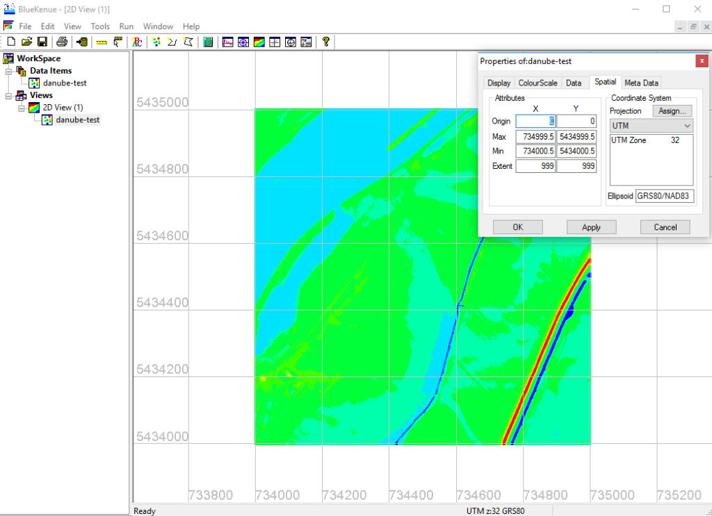
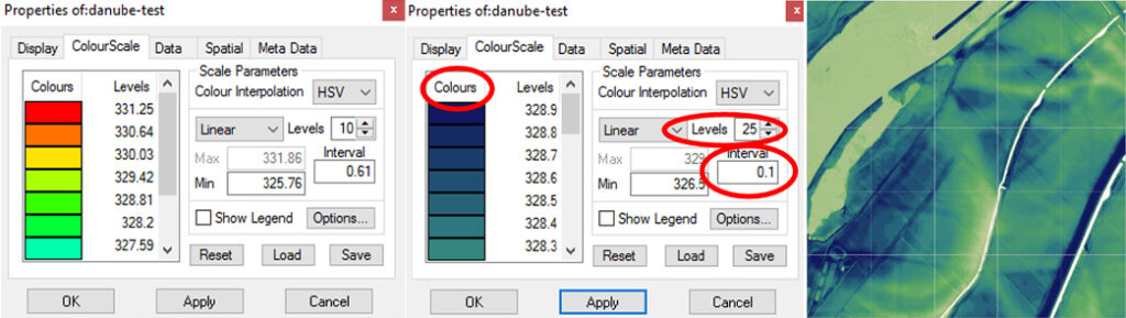
Then start the meshing process by drawing a model boundary line.

1. Click the “New Closed Line” symbol in the toolbar. A little square appears next to your mouse pointer. Draw a polygon in the “2D View (1)” window delineating your model area. The area of interest is the pilot area field plot. End the delineation by pressing “Esc”.
2. Name the closed line “model-outline”, skip all other options and press “OK”.
3. Save “model-outline” by highlighting it in the “WorkSpace” and clicking on the disc symbol.
4. Click on “File -> New…-> T3 Mesh Generator”. In the pop-up window enable “Resample Outline”, set the “Default Edge Length” to 0.5 m, or finer, but at maximum the resolution of your input data and press “OK”. High-resolution input data (i.e. at least 0.5 m DEM resolution) is critical here, because otherwise the mesh will not accurately represent the terrain complexity relevant for modelling soil erosion.
5. Drag the previously created “model-outline” object on the “Outline” of the “newT3Mesh” (see arrow in Figure 3).
6. Double-click the “newT3Mesh” and click “Run”, then “OK” and after finishing the meshing process “OK”. Rename the “New Mesh” to “T3-Mesh”.
7. To check your mesh pull it on the section “2D Views” under “Views”.

SELAFIN Object Creation

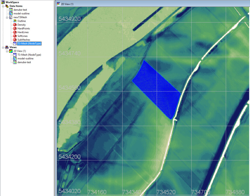
To start with the SELAFIN object creation, you need BlueKenueTM with the .xyz file and the “T3-Mesh” loaded. You can then create the SELAFIN object by:

1. Click “File -> New -> SELAFIN Object…”. A “newSelafin” object appears in the “Data Items” panel. Right-click the “newSelafin” object and select “Add variable…”.
2. Select “T3-Mesh” as your mesh, in the “Name” field select “BOTTOM”, in the “Units” field select “M”. Then click “OK”.
3. Save the SELAFIN object, e.g. as “SELAFIN.slf”.

As the created SELAFIN object lacks elevation data, you should add it now:

1. Click “File -> New -> 2D Interpolator…”. A “newInterpolator2D” object will appear in the “Data Items” panel. Then drag the DEM onto “newInterpolator2D” (see Figure 4).
2. Highlight the “BOTTOM” attribute of your previously created SELAFIN object. With the attribute highlighted go to “Tools -> Map Object…”. Select the object “newInterpolator2D”. Then click on “OK” once the process is finished.
3. Save “BOTTOM” as a mesh. Save “SELAFIN” as a SELAFIN object, e.g. as “SELAFIN.slf” to overwrite your previous SELAFIN object.
4. To check, whether the elevation interpolation worked correctly, drag the “BOTTOM” mesh on the section “2D Views” under “Views”.

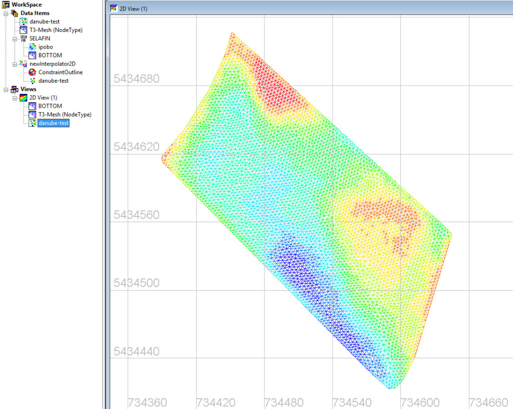
Furthermore, roughness needs to defined for the fields/plots so that the roughness’ influence on erosion processes can be taken into account. Here, chose to work with Manning’s roughness nm. for easy understanding: higher values for Manning’s nm means higher roughness. If the fields/plots do not have uniform roughness, the roughness is defined by allocating roughness zones:

1. For this purpose, use Blue Kenue™’s “New Closed Line” option and delineate the different roughness zones of the mesh.
2. When your closed line is finished press “Escape” and assign a roughness value in the appearing pop-up window.
3. Save all roughness zones as individual files.
4. Then select “File->New->2D Interpolator…”. The new interpolator appears in the “WorkSpace”.
5. Pull the previously created closed lines onto the interpolator.
6. Add a new variable to your SELAFIN object by right-clicking it and selecting “Add Variable…”. In the pop-up window choose “BOTTOM FRICTION” as name and Manning as unit. Enter 0.03 as “Default Node Value”.
7. To interpolate the friction values on the mesh highlight the variable “BOTTOM FRICTION”, go to “Tools->Map Object…” select the “new 2D Interpolator” and click “OK”. A processing pop-up window appears. Then, when processing is finished click “OK”.
8. To check your interpolation, pull the “BOTTOM FRICTION” on the section “2D Views” under “Views”. It might be necessary to adjust the “ColourScale” and change the minimum of the “ColourScale” to 0. Save the SELAFIN object, e.g. as “SELAFIN-friction.slf”.

Boundary Conditions

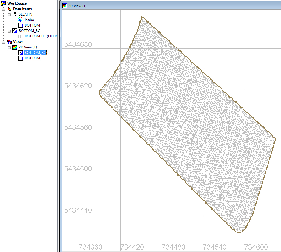
TELEMAC needs to know how to handle the outer edges of the mesh, and in this special use case, also potentially internal mesh nodes where discharge originates in the form of (intense) rainfall per time. These source nodes, together with the nodes through which water flows out of the model (i.e. the nodes at the lowest elevation edges), represent the “liquid boundaries” of the mesh. These exist alongside the outer-edge mesh nodes through which no water flows (“solid boundaries”). For this purpose, a .cli boundary file needs to be created using BlueKenueTM. The first step towards the .cli file is to create an object that constitutes all outer boundary nodes of the mesh:

1. Click “File->New->Boundary Conditions (Conlim)…” In the pop-up window, select the previously created “BOTTOM” mesh and click “OK”.
2. A new “BOTTOM_BC” object appears in the “Data Items” panel.
3. To check the newly created Conlim object, pull it on the section “2D Views” under “Views” (see Figure 5)
4. Save the Conlim object, e.g. as “boundaries.bc2”.

Next, liquid boundaries need to be defined by allocating water input and output nodes. The default type of boundary is “closed boundary (wall)”. Therefore, change the boundary type of both, input and output boundaries:

1. Locate the nodes for input/output boundary.
2. Double-click one of the input/output nodes and hold the shift key to add more nodes to your boundary. Right-click on the nodes that are now highlighted in purple and select “Add Boundary Segment”.
3. In the opening window “CONLIM Boundary Segment Editor” define a boundary name and boundary code (e.g. 4-5-6, this will be specified based on the development for the German pilot areas). Click “OK”. Save your input/output boundary by overwriting your “boundaries.bc2” file.
4. Create a .cli file by highlighting the “boundaries (LIBHOR)” entry of the boundaries object and saving it, for example “boundaries.cli”

Steering file setup

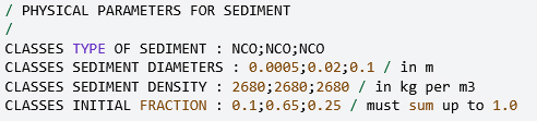
A default steering file (.cas) is provided by PP4-IWS during the project, based on the German pilot areas. To tailor the steering file for their pilot areas, other PPs can adjust the following keywords in the steering file by opening it in a text editor:

• Adjust the simulation title (TITLE : ‘Your-pilot-area’)
• In the section “Computation Environment” adjust names of the case study or simulation files (.cli, .slf and zonal roughness, if applicable)
• Ensure the boundary order is correct but do not change the boundary type: The order of open boundaries can be read from the .cli file. The first open boundary that is listed in the .cli file corresponds to the first list element in any “PRESCRIBED…” keyword. An open boundary node in the .cli file is characterized by a line beginning with a boundary code different from 2-2-2 (as, e.g. 4-5-6). BlueKenue also marks the names of open boundaries at the line ends (after the hashtag).
• In-file adjustment of the global roughness: The keyword “LAW OF THE BOTTOM FRICTION” is used to define a friction law for topographic boundaries. Set it to “4” which corresponds to Manning’s roughness nm, or alternatively, “5” (Nikuradse) to prescribe a physically meaningful characteristic roughness length (typically have of the height of tillage furrows). With the keyword, “FRICTION COEFFICIENT FOR THE BOTTOM” a roughness coefficient can be specified, which corresponds to the calibration parameter for tillage, soil type, crop type and growth stage of your pilot area and its environmental conditions. For further information on calibration see Chapter 6.
• Adjustment of grain size parameters and cohesion (GAIA): Gaia considers sediment with grain diameters of less than 60∙10-6 m to 100∙10-6 m being cohesive. To model such fine sediment, where capillary forces may have significant effects on erosion, adaptations in the boundary conditions file and types are required. In the cohesive sediment case, the “TYPE OF SEDIMENT” keyword is “CO”. In general, GAIA enables the differentiation between classes of sediment diameters with the keyword “CLASSES SEDIMENT DIAMETERS”. Additionally sediment density can be added to each sediment classes with the keyword “CLASSES SEDIMENT DENSITY”. The keyword “CLASSES INITIAL FRACTION” assigns a fraction to each of the defined sediment classes. An example of the section “PHYSICAL PARAMETERS FOR SEDIMENT” in the .cas file is given in Figure 6.

4. Numerical Simulations

The numerical modelling chapter gives instructions on how to run the numerical modelling system and gain insights from the simulation results (post-processing).

All input files need to be correctly stored in the dedicated simulation folder “pilot-area” on the VM, as defined in the pre-processing chapter. Then navigate (“cd”) to the Telemac configuration folder and load the Telemac environment:

Navigate to the dedicated simulation folder and run the steering file:

Depending on the provided computational resources (CPU, RAM), the simulation can take several hours or even days, before the end of a successful computation is indicated with the line “My work is done” in Linux Terminal (i.e. within the VirtualBox).

5. Post-processing

Export Simulation Results

The result files will be saved in the simulation folder as “rdanube.slf” and “rdanubeGAIA.slf”. They can now be opened in QGIS for visualization.

Visualization of mesh data in QGIS

Open QGIS, create a new project and refer to the relevant section for guidance on working with mesh files, background maps, scrolling through timesteps, and exporting graphics.

Loading a Selafin (.slf) mesh

To load a Selafin object into QGIS:

1. Add the layer by clicking “Layer->Add Layer->Add Mesh Layer…”. Browse to the .slf file. The QGIS’ mesh provider (MDAL) recognises Selafin (slf) natively, so the grid and all result datasets appear in one click. Additionally, a layer styling window opens on the right hand side.
2. If your mesh rendered correctly, a new “Mesh” entry is created in the Layers panel.

Adding an OpenStreetMap backdrop

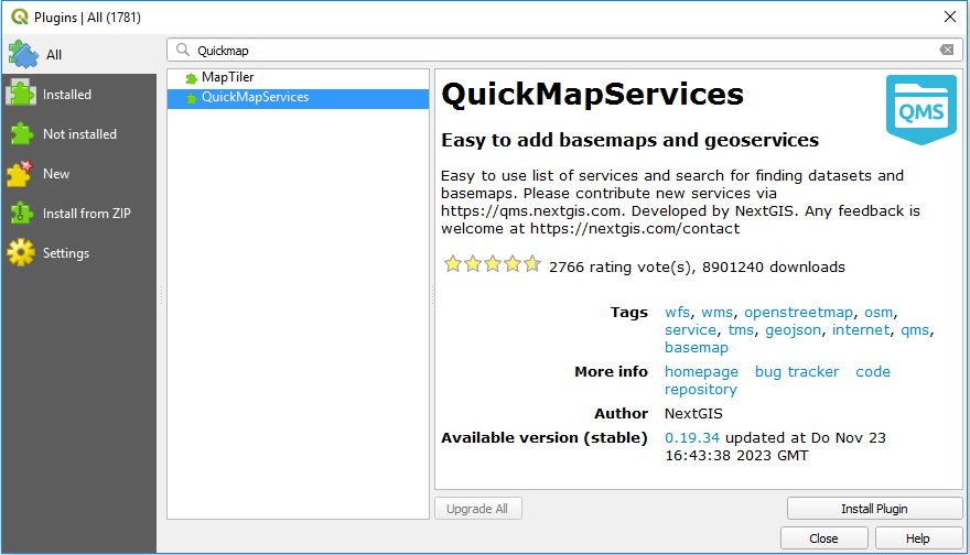
To add an OpendStreetMap backdrop to QGIS:

1. Under “Plugins->Manage and Install Plugins…” install the “QuickMapServices” plugin (see Figure 7).
2. Click “OSM Standard” or any other XYZ tile to drop a georeferenced basemap beneath the mesh in the “Layer” panel.

Verification of results & reporting of roughness values

Mesh layers are automatically “temporal”. You can view different timesteps by adjusting viewing options:

1. Enable the temporal controller option under “View -> Panels -> Temporal Controller”
2. Click “Set to Full Range” (see Figure 8).
3. Then play, step or drag the slider to move through simulation time.

The rainfall simulations represent unsteady runs that export many timesteps, which enable to explore different stages of a rainfall event and different parameters.

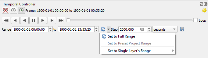
The Telemac output files contain results for several parameters. For analysing parameters, switch between them:

1. Hit “F7 ‘(Layer Styling” or double click the mesh layer to open “Properties->Symbology/Datasets”. Here, each dataset group (water depth, velocity magnitude, bed change, erosion/deposition, etc.) is listed.
2. Click the icon next to the parameter to activate a parameter and QGIS repaints it instantly.
3. Vector arrows (for velocities) or contours can be toggled and colour ramps adjusted in the same panel.

The simulated erosion / deposition rates can be explored by analysing the “bottom elevation” parameter. If the simulated bottom elevation at the end of the simulation does not match observed erosion, roughness coefficients need to be adjusted. This roughness correction is expected, as crop type, growth stage and tillage affect how much the surface runoff slows down as a result of these parameters. If the simulated erosion is too high, roughness should be increased to slow down the flow and therefore its capacity of eroding sediment. Vice versa, if the simulated erosion is too low, roughness should be reduced. Moreover, in the case of cohesive sediment, cohesion properties might need to be changed, as those can substantially affect erosion. This is why calibration also is a function of soil types, beyond crop type, growth stage and tillage. Finally, report the optimum values for roughness and cohesiveness to the project table prepared by PP4-IWS.

Saving a high-resolution figure

For further results analysis and result communication, save your simulated parameters individually as high-resolution figures:

1. Open “Project->New Print Layout”. Add a map frame and any legend/scale bar.
2. Press “Export as Image”. Choose “JPEG” and set a resolution of 300-500 dpi or a custom pixel size for publication quality output.
3. QGIS writes both, the .jpg and an optional world-file, if georeferencing is ticked.

6. Calibration

Purpose of model calibration

Calibration involves the step-wise adaptation of model input parameters to yield a possibly best (statistic) fit of modelled and measured data. In the process of model calibration, only one parameter should be modified at a time by 10 to 20-% deviations from its default value. In this project, the calibration parameter is roughness that can be expressed in term of beginning Manning’s nm or equivalent sand roughness ks. The higher the roughness parameter, the higher is the friction induced by the terrain on the flow. Thus, high roughness means lower flow velocity and less erosion; on the contrary, low roughness means higher flow velocity and more erosion. For instance, if in the beginning Manning’s nm= 0.03, the calibration may test for Manning’s nm= 0.033 (if the model overpredicts erosion) or Manning’s nm= 0.027 (if the model underpredicts erosion), ultimately to find out which value for Manning’s nm brings the model results closest to observations, as a function of tillage, crop type and crop growth.

Model calibration process

The modelled erosion rates can be compared to the difference between two DEMs of the project area: the base DEM that is used as input DEM for modelling and an additional DEM that is measured in the project area after observing the (modelled) extreme event. The difference between the two DEMs is called “DEM of Differences – DoD”. The numerical model initially runs with an initial guess for the roughness value (typically 0.05 for agricultural fields with shallow overflows) to simulate an erosive rainfall event that caused the terrain to change from the first to the second DEM by dz defined in the DoD. Thus, roughness is adjusted, that is, calibrated to match the observed and modelled DoD. The target accuracy is that modelled and observed DoDs have no more than 20% difference, when calculating the

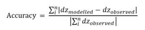
where subscript i refers to the dz-pixel under consideration and 𝑛 is the total number of pixels of the DoD raster.

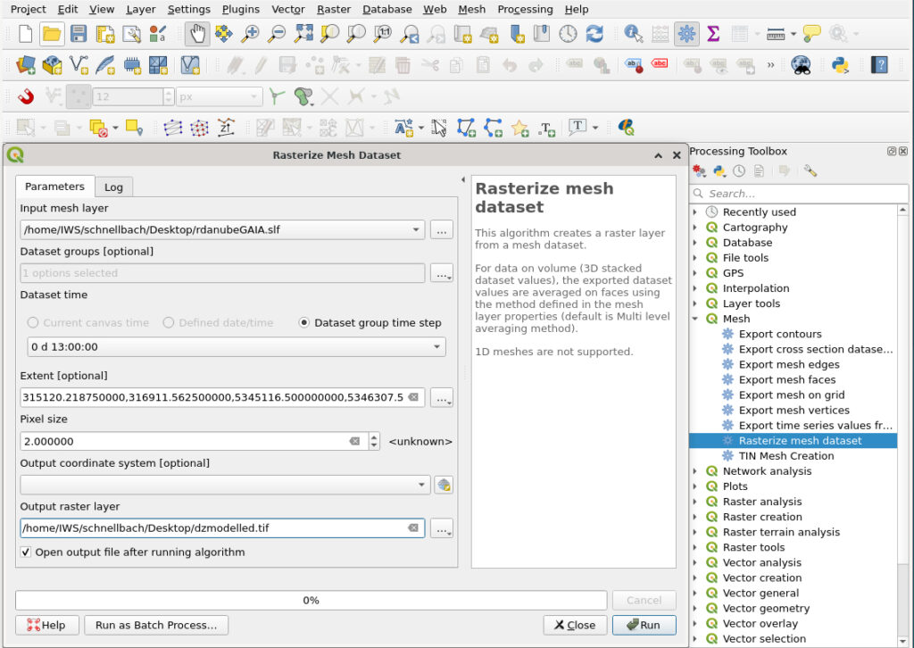
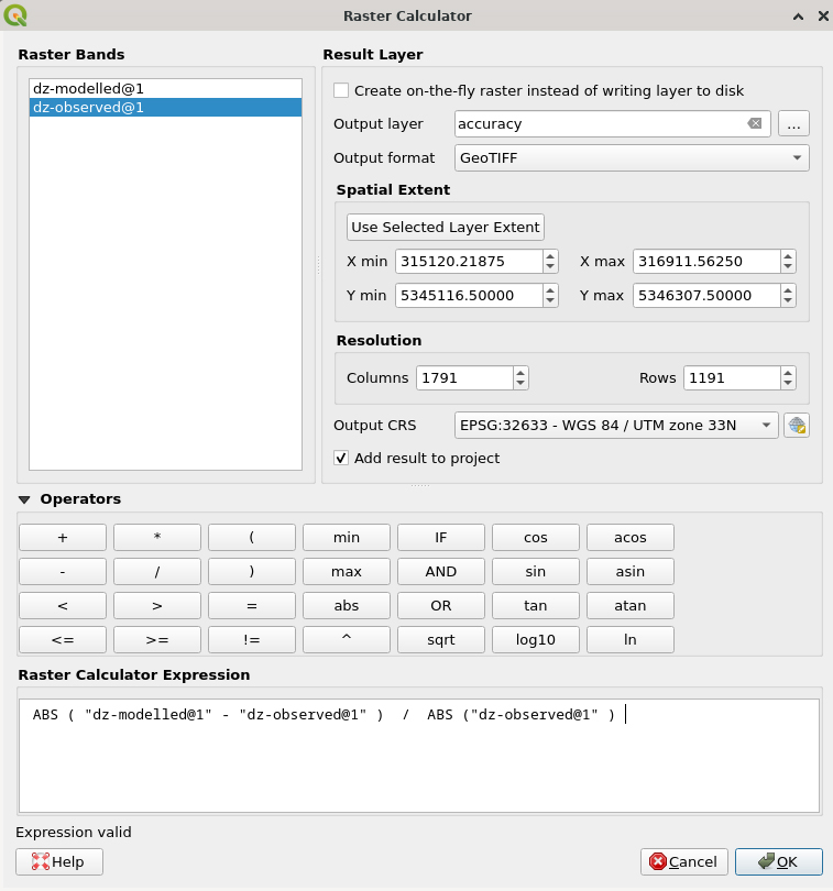
The calculation of accuracy can be performed by first extracting the modelled DoD from the Telemac output mesh (.slf) in GeoTIFF format (see Figure 9), and then using raster calculator functions (“RasterRaster Calculator…”) in QGIS (see Figure 10).

To calibrate the roughness value, modify the friction coefficients in the Telemac steering file (.cas), so that the 𝐴𝑐𝑐𝑢𝑟𝑎𝑐𝑦 is optimised. Report the friction (roughness) coefficients, so that PP4-IWS can generate calibration tables with specific friction (roughness) coefficients for tillage methods and crop types.

Resources

This chapter gives an overview of the resources provided by IWS for numerical modelling and provides resources for further insights.

Provided Files

IWS-PP4 currently provides three files on the Project’s Google Drive for Project Partners to start the numerical modelling process for their pilot areas:

• D.1.1.1: Guidance for Numerical Model Usage (this document);
• the VM as an .ova file.

The following files are provided successively on the project’s Google Drive:

• Telemac steering files;
• Telemac example file.

Literature (further reading)

Telemac2D manual: https://gitlab.pam-retd.fr/otm/telemac-mascaret/-/blob/v9.0.0/documentation/telemac2d/user/telemac2d_user_9.0.pdf

GAIA reference manual: https://gitlab.pam-retd.fr/otm/telemac-mascaret/-/raw/v9.0.0/documentation/gaia/reference/gaia_reference_9.0.pdf

Hydro-Informatics.com: https://hydro-informatics.com